4 Method
The CyIPT is a big data project, meaning much of the work involved accessing, collating, cleaning and pre-processing data. The initial plan was to build CyIPT completely for a single region (Bristol) before creating a national version. In practice, it became clear that time was better invested in ‘optimising early’ to create methods that would scale nationally from the beginning. This meant that, although we did use Bristol as the main case study city, we were aiming to create a nationally-scalable product all along, avoiding problems associated with scaling-up later down the line.
This involved working with software for handling OSM data such as the osmdata R package (Padgham et al. 2017) and ‘simple features’, a new class system for spatial data in the R programming language (R Core Team 2017).
OpenStreetMap (OSM) data was downloaded in bulk and a much work was put into cleaning the user-contributed metadata (known as ‘tags’) that define road type and other features. The decision to use OpenStreetMap, rather an alternatives such as Ordnance Survey data, was due to the higher levels of detail about cycling networks provided in OSM, and the flexible and open licencing terms of OSM data.
A major challenge early on was the calculation of road widths, or rather the width of road space available to construct new cycle infrastructure. To visualise the availability/unavailability of street space the website streetmix.net (see Figure 4.1). Although promising for visualising roads on a one-by-one basis, we decided not to streetmix in the final version because we could not find ways to automate the production of road width types.
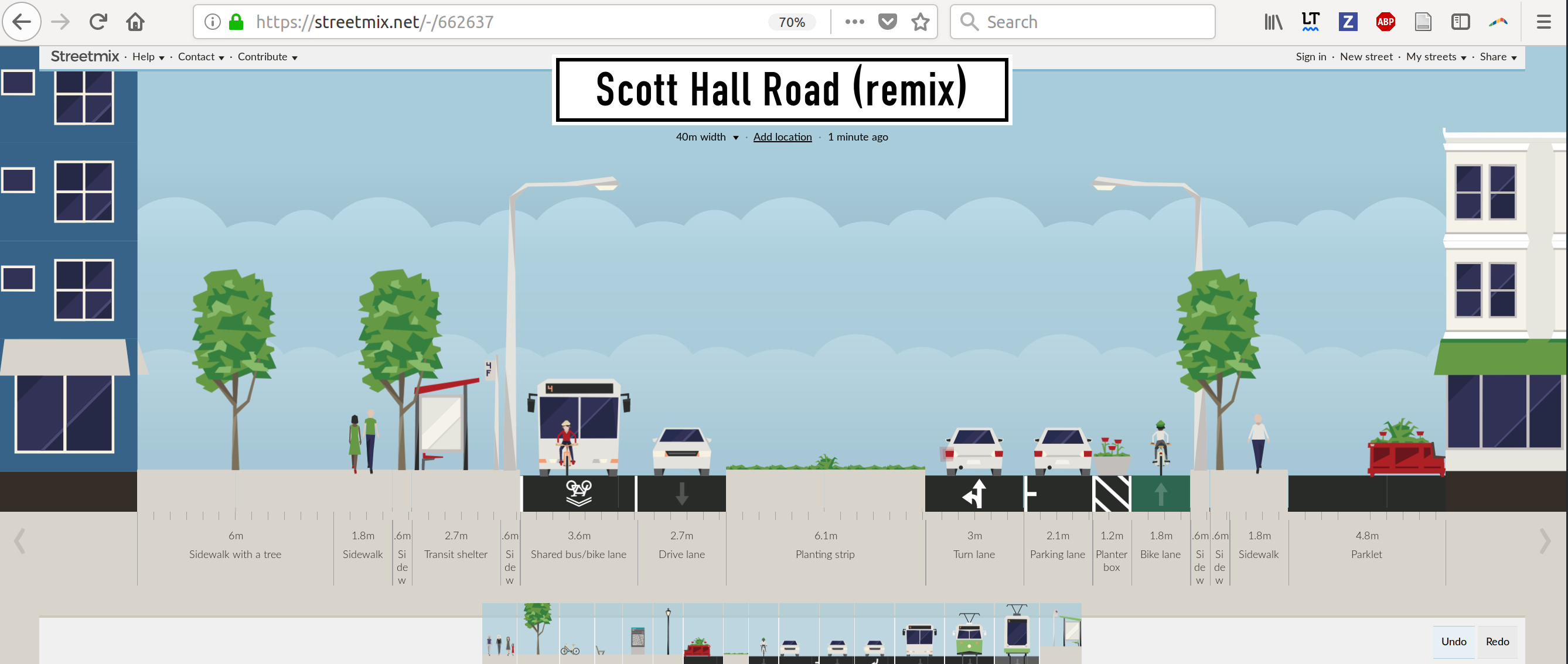
Figure 4.1: Example visualisation from the streetmix website. Could this be a way to help stakeholders assess width constraints?
To overcome the road-widths challenge we turned to Ordnance Survey (OS) data. The CyIPT Team has access to a 2005 copy of the OS MasterMap for England. The code was developed to measure the width of the road polygon in the MasterMap and assign that value to the line representation of the road in the OSM.
To make the results intuitive and avoid any potential licencing issues with OS data, the results of these calculations are presented approximately and in relation to new infrastructure, ranging from “Insufficient” to “More than sufficient” width (see the CyIPT Manual, section 4.6).
Another major challenge was the estimation of uptake following new infrastructure. It is well known that building appropriate infrastructure (protected cycleways) in appropriate places can lead to dramatic uptake of cycling, as illustrated by the example of Seville, Spain, which we use here by way of a comparative example. Despite high temperatures there, cycling levels in the city quadrupled following investment in a carefully planned route network (illustrated in Figure 4.2) from less than 2% before 2006 to more than 8% (in the survey month of November) following infrastructure investment (Marqu’es et al. 2015). This network represents around 0.3 m of segregated cycle infrastructure per person (~200 km divided among the city’s ~700,000 people).

Figure 4.2: The core cycling network in Seville, composed of the basic (77 km) and complementary (120 km) protected cycle path network, which led to cycling increasing fourfold.
Translating knowledge of the success of Seville’s infrastructure provision into practice is not a simple process. A simplistic approach would be to divide the increase in cycling levels (around 6 percentage points) by the length of new infrastructure (around 200 km), which would imply that new infrastructure leads to cycling uptake at a rate of around one percentage point per 30 km of cycling provision.
Assuming this relationship found in Seville holds everywhere would be naïve, not only due to cultural differences between the UK and Spain but also due to a number of measurable differences between paths constructed in one place that may not apply in another:
- Level of cycling potential: clearly a cycle path constructed where there is high latent demand will attract more users than a path constructed where there is little demand.
- Type of infrastructure: high quality, wide, cycleways offering protection from motor traffic can be expected to have a greater impact on cycling levels than thin unprotected cycle lanes, for example.
- The conditions on the rest of the route beyond the interventions are likely to play a role. For example, cycling infrastructure that allows a cyclist to avoid busy roads is likely to generate more uptake than infrastructure that substitutes for existing quiet 20mph streets.
Each of these factors was accounted for using an uptake model that used historic interventions (between 2011 and 2001) to predict change in cycling between the 2001 and 2011 census, at the MSOA origin-destination level. An illustration of the input datasets that allowed this model is presented at the regional level in Figure 4.3.

Figure 4.3: Illustration of the relationship between infrastructure creation (2001 - 2011 - source Sustrans and Transport Direct) and change in cycling levels over the same period (source: origin-destination data from Wicid). Named regions had levels of cycling uptake and levels of infrastructure provision above the median.
Figure 4.4 illustrates how the data look at the local level, with individual origin-destination pairs ‘exposed’ to infrastructure clear from where they crossed the grey blobs (representing interventions). The fact that the dependent variable (cycling uptake) operates at a different level from the primary dependent variable (new cycling infrastructure) poses a question: how to measure ‘exposure’ to new infrastructure?
A number of approaches were tested, including the length of infrastructure within a buffer of the straight line representing each OD pair, and the average proximity to new infrastructure for each OD pair. In the end, however, a more narrow definition of exposure was used: length of new infrastructure present on the fastest route for each OD pair. Although more restrictive, this definition had the advantage that it was directly applicable to the input data used by CyIPT. Furthermore, it allowed additional variables such as the percentage of the trip after an intervention that could be made on roads with low speed limits. It was found that low speed limits of the route were a powerful predictor of cycling uptake following new infrastructure. To model this the percentage of the route at different speed limits was used as an interaction variable that diminished the effectiveness of new infrastructure for fast (40mph+) roads and increased the effectiveness of new infrastructure in cases where the percentage of the route that was on low speed limit roads was high.

Figure 4.4: Illustration of the input data at the local level in Bristol.
(The reference in the above paragraph to the ‘fastest route’ refers to the modelling of likely cyclist route preferences available from the CycleStreets cycle journey planner. This system provides a set of suggested routes for each A-B OD pair, in the form of a fastest route, quietest route, and a balanced route between these. Such routes are also used by the Propensity to Cycle Tool. Ongoing improvements in the routing engine modelling were made during the CyIPT work, reflecting the importance of aiming for maximum accuracy of these routes.)
One of the input datasets used in the uptake model was a newly-available dataset liberated by CycleStreets as part of the project. The DfT England Cycling Data project was an initative in 2011 to convert data collected for the (now-defunct) Transport Direct cycle journey planner project and make it available for use in OpenStreetMap. This data had not hitherto been released, but conversion work within the CyIPT project has now enabled this dataset to become publicly available using open standards (GeoJSON), maximising taxpayer value for this data.
To present the results of the uptake model on the map user interface, a slider was used to allow the user to select how much funding they had available per scheme. A drop-down menu was added to enable the user to filter-out schemes depending on their associated BCRs. This method of selecting schemes can be used to interactively identify worthwhile schemes in the city of interest, with promising schemes for Bristol illustrated in Figure 4.5.
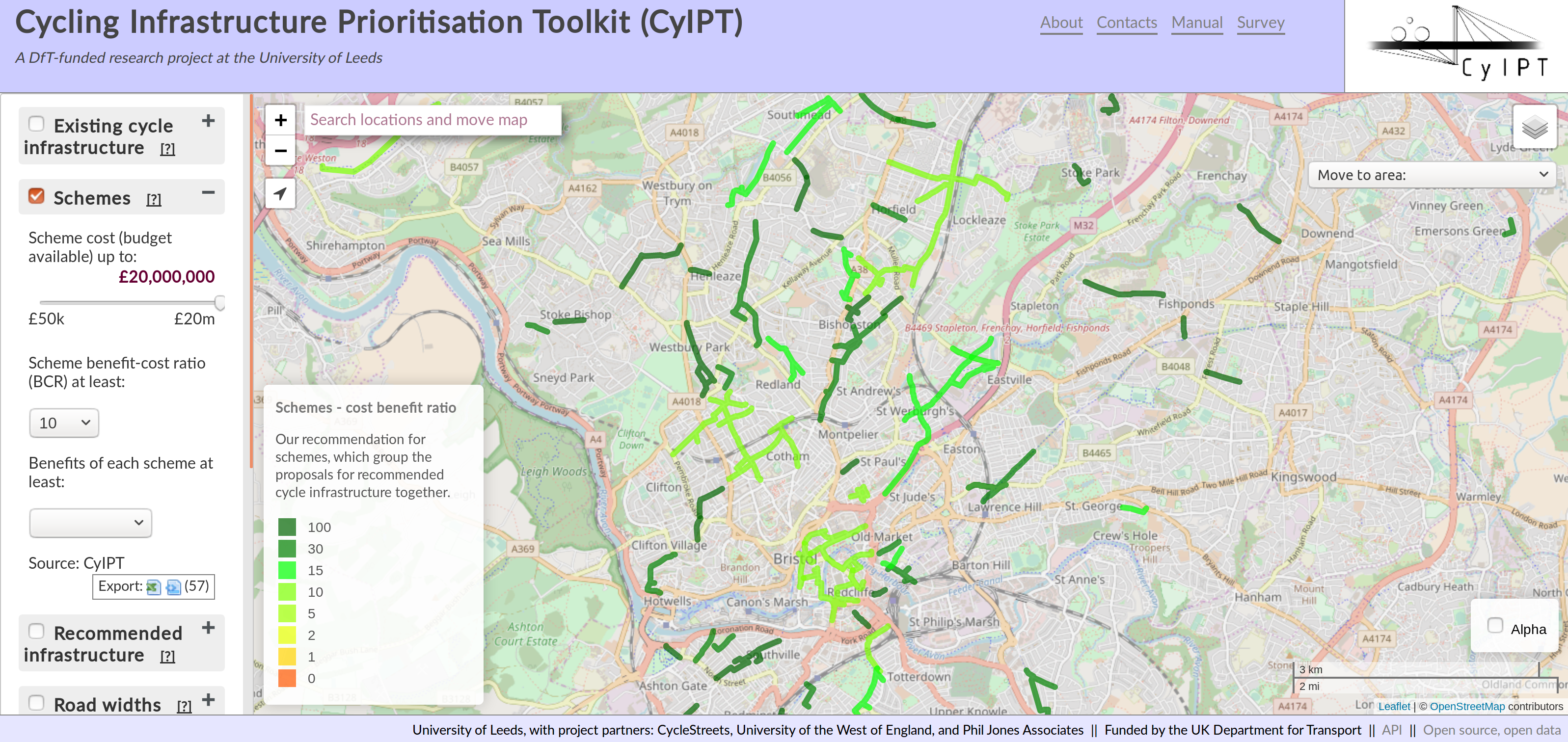
Figure 4.5: Schemes with high estimated BCRs illustrated for Bristol, selected using the BCR dropdown menu in the Schemes layer.
References
Padgham, Mark, Robin Lovelace, Maëlle Salmon, and Bob Rudis. 2017. “Osmdata.” The Journal of Open Source Software 2 (14). doi:10.21105/joss.00305.
R Core Team. 2017. R: A Language and Environment for Statistical Computing. Vienna, Austria: R Foundation for Statistical Computing. https://www.R-project.org/.
Marqu’es, R., V. Hern’andez-Herrador, M. Calvo-Salazar, and J.A. Garc’ia-Cebri’an. 2015. “How Infrastructure Can Promote Cycling in Cities: Lessons from Seville.” Research in Transportation Economics 53 (November): 31–44. doi:10.1016/j.retrec.2015.10.017.